Data Mining: Assignment 1
The goal of this project is to build a CIFAR-10 image classifier using pytorch and tensorflow. In this project, different classifiers are built for the purposes of comparisons.
To compare the performances among the fitted models, we will use the predicted accuracy and the estimated loss of each model as comparison metric. We will also plot graphs of accuracies and estimated losses against the fitted models for easy comparisons. The performances of each model will also be evaluated based on the test data.
The layout of this project is organized as follows; in section 1, we import the require libraries and data necessary for this project. We also report the dimensions of the dataset, both the training and the testing set, and also normalize the dataset. In section 2, we will fit 5 different models using tensorflow and perform a classification report for each class in the test data using the optimal model. In section 3, 3 different models will also be fitted using pytorch and classification reports for each class based on the test data will also be computed. In section 4, we will select our overall optimal model, and also plot graphs of the accuracies and the losses against each model for easy comparison and visualization. Finally in Section 5, we end our discussion by some concluding remarks and contributions.
1.0 Libraries
import torch
import torchvision
import torchvision.transforms as transforms
import matplotlib.pyplot as plt
import numpy as np
import torch.nn as nn
import torch.nn.functional as F
import torch.optim as optim
import tensorflow as tf
from tensorflow.keras import datasets, layers, models
from keras.preprocessing.image import ImageDataGenerator
from sklearn.metrics import confusion_matrix, classification_report
from matplotlib import pyplot
1.1 Import Dataset
In this project, we will use the CIFAR10 dataset. This data has about 60000 images of the following classes: ‘airplane’, ‘automobile’, ‘bird’, ‘cat’, ‘deer’, ‘dog’, ‘frog’, ‘horse’, ‘ship’, ‘truck’. The images in the CIFAR-10 dataset are of size 3x32x32, that is, 3-channel color images of size 32x32 pixels. In this project, we will split the dataset into training set and testing set. The split ratio is 80% training set, which will be used to train our classifier, and 20% testing set, which will be used to validate our trained model.
Reference: The reference code for this project can be obtained from the following links:
Pytorch:
- https://pytorch.org/tutorials/beginner/blitz/neural_networks_tutorial.html
- https://pytorch.org/docs/stable/generated/torch.nn.Module.html#torch.nn.Module
Tensorflow:
- https://machinelearningmastery.com/category/deep-learning/page/7/
- https://www.youtube.com/watch?v=7HPwo4wnJeA&t=24s
# Import data: This data will be used to build the classifier using pytorch
transform = transforms.Compose(
    [transforms.ToTensor(),
     transforms.Normalize((0.5, 0.5, 0.5), (0.5, 0.5, 0.5))])

batch_size = 5

trainset = torchvision.datasets.CIFAR10(root='./data', train=True,
                                        download=True, transform=transform)
trainloader = torch.utils.data.DataLoader(trainset, batch_size=batch_size,
                                          shuffle=True, num_workers=2)

testset = torchvision.datasets.CIFAR10(root='./data', train=False,
                                       download=True, transform=transform)
testloader = torch.utils.data.DataLoader(testset, batch_size=batch_size,
                                         shuffle=False, num_workers=2)
Files already downloaded and verified
Files already downloaded and verified
#Import data: This data will be use build the classifier under tensorflow
(x_train, y_train), (x_test, y_test) = datasets.cifar10.load_data()
Data Structure and Dimension
x_train.shape
(50000, 32, 32, 3)
x_test.shape
(10000, 32, 32, 3)
y_train = y_train.reshape(-1,)
y_train[:5]
array([6, 9, 9, 4, 1], dtype=uint8)
# Image classes of the dataset
classes = ('plane', 'car', 'bird', 'cat','deer', 'dog', 'frog', 'horse', 'ship', 'truck')
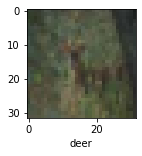
# Display an image of from the train data
def plot_sample(x, y, index) :
    plt.figure(figsize = (15, 2))
    plt.imshow(x[index])
    plt.xlabel(classes[y[index]])
plot_sample(x_train, y_train, 10)
# Display some 5 random training images
def imshow(img):
    img = img / 2 + 0.5     # unnormalize
    npimg = img.numpy()
    plt.imshow(np.transpose(npimg, (1, 2, 0)))
    plt.show()

dataiter = iter(trainloader)
images, labels = dataiter.next()

# show images
imshow(torchvision.utils.make_grid(images))
# print labels
print(' '.join('%5s' % classes[labels[j]] for j in range(batch_size)))
dog frog frog truck ship
1.2 Normalize Dataset
We normalized the dataset, both the train and test, to take values between 0 and 1.
x_train = x_train / 255
x_test = x_test / 255
2.0 Training the classifier using tensorflow
The following five different classifiers are trained in this section using tensorflow;
- 2 simple 2-convolutional layer classifiers with different filter sizes
- 3 3-convolutional layer classifiers with different numbers of fully connected layers and filter sizes. The input shape for each classifier in this section is 32X32X3, and the ReLu activation is used in the input layer for each classifier. For all classifiers in this category, the “Adam” optimizer and the sparse categorical cross-entropy loss are used. “Softmax” is used as activation in the output layer. Epochs for all classifiers is set at 10.
2.1 Train a 2-layer CNN Model
cnn1 = models.Sequential([
    #cnn
    layers.Conv2D(filters = 64, kernel_size = (3, 3), activation = 'relu', input_shape = (32, 32, 3)),
    layers.MaxPooling2D((2,2)),

    layers.Conv2D(filters=128, kernel_size=(3, 3), activation='relu'),
    layers.MaxPooling2D((2,2)),

    #dense
    layers.Flatten(),
    layers.Dense(128, activation='relu'),
    layers.Dense(10, activation='softmax')]
)

cnn1.compile(optimizer = 'adam',
            loss = 'sparse_categorical_crossentropy',
            metrics = ['accuracy'])
cnn2 = tf.keras.models.Sequential()
cnn2.add(tf.keras.layers.Conv2D(filters=32, kernel_size=3, activation='relu', input_shape=[32, 32, 3]))
cnn2.add(tf.keras.layers.MaxPool2D(2, 2))
cnn2.add(tf.keras.layers.Conv2D(filters=32, kernel_size=3, activation='relu'))
cnn2.add(tf.keras.layers.MaxPool2D(2, 2))
cnn2.add(tf.keras.layers.Flatten())
cnn2.add(tf.keras.layers.Dense(units=128, activation='relu'))
cnn2.add(tf.keras.layers.Dense(units=10, activation='softmax'))

cnn2.compile(optimizer = 'adam',
             loss = 'sparse_categorical_crossentropy',
             metrics = ['accuracy'])
2.1.1 Test Model
For the 2-convolutional layer networw, it turns out that classifier 1 (CNN-1) has an accuracy rate of 71.3% and a loss of 0.854 on the test test data whiles classifier 2 (CNN-2) has an accuracy rate of 68% and a loss of 0.927 from the same test data. This implies CNN-1 has outperformed CNN-2. See the results below.
cnn1.fit(x_train, y_train, epochs=5)
Epoch 1/5
1563/1563 [==============================] - 43s 27ms/step - loss: 1.3668 - accuracy: 0.5096
Epoch 2/5
1563/1563 [==============================] - 42s 27ms/step - loss: 1.0084 - accuracy: 0.6495
Epoch 3/5
1563/1563 [==============================] - 43s 27ms/step - loss: 0.8632 - accuracy: 0.6991
Epoch 4/5
1563/1563 [==============================] - 44s 28ms/step - loss: 0.7543 - accuracy: 0.7388
Epoch 5/5
1563/1563 [==============================] - 44s 28ms/step - loss: 0.6666 - accuracy: 0.7696


<keras.callbacks.History at 0x7f9ba2355880>
cnn1.evaluate(x_test, y_test)
313/313 [==============================] - 2s 6ms/step - loss: 0.8540 - accuracy: 0.7133


[0.8540308475494385, 0.7132999897003174]
cnn2.fit(x_train, y_train, epochs=5)
Epoch 1/5
1563/1563 [==============================] - 23s 13ms/step - loss: 1.4661 - accuracy: 0.4715
Epoch 2/5
1563/1563 [==============================] - 19s 12ms/step - loss: 1.1301 - accuracy: 0.6024
Epoch 3/5
1563/1563 [==============================] - 20s 13ms/step - loss: 0.9946 - accuracy: 0.6532
Epoch 4/5
1563/1563 [==============================] - 20s 13ms/step - loss: 0.9033 - accuracy: 0.6846
Epoch 5/5
1563/1563 [==============================] - 20s 13ms/step - loss: 0.8271 - accuracy: 0.7118


<keras.callbacks.History at 0x7f9b888151f0>
cnn2.evaluate(x_test, y_test)
313/313 [==============================] - 1s 3ms/step - loss: 0.9267 - accuracy: 0.6800


[0.9266972541809082, 0.6800000071525574]
2.2.0 Train a 3-layer CNN Model.
Classifier 3 (CNN-3) below is a 3-convolutional layer with 2 fully connected layers, classifier 4 (CNN-4) below is a 3-convolutional layer with 3 fully connected layers, and classifier 5 (CNN-5) below is a 3-convolutional layer with 3 fully connected layers. Different filter sizes are used to fit each classifier.
cnn3 = models.Sequential([
    #cnn
    layers.Conv2D(filters = 64, kernel_size = (3, 3), activation = 'relu', input_shape = (32, 32, 3)),
    layers.MaxPooling2D((2,2)),

    layers.Conv2D(filters=128, kernel_size=(3, 3), activation='relu'),
    layers.MaxPooling2D((2,2)),

    layers.Conv2D(filters=256, kernel_size=(3, 3), activation='relu'),
    layers.MaxPooling2D((2,2)),

    #dense
    layers.Flatten(),
    layers.Dense(120, activation='relu'),
    layers.Dense(64, activation='relu'),
    layers.Dense(10, activation='softmax')]
)

cnn3.compile(optimizer = 'adam',
             loss = 'sparse_categorical_crossentropy',
             metrics = ['accuracy'])
cnn4 = models.Sequential([
    #cnn
    layers.Conv2D(filters = 64, kernel_size = (3, 3), activation = 'relu', input_shape = (32, 32, 3)),
    layers.MaxPooling2D((2,2)),

    layers.Conv2D(filters=128, kernel_size=(3, 3), activation='relu'),
    layers.MaxPooling2D((2,2)),

    layers.Conv2D(filters=256, kernel_size=(3, 3), activation='relu'),
    layers.MaxPooling2D((2,2)),

    #dense
    layers.Flatten(),
    layers.Dense(256, activation='relu'),
    layers.Dense(120, activation='relu'),
    layers.Dense(64, activation='relu'),
    layers.Dense(10, activation='softmax')]
)

cnn4.compile(optimizer = 'adam',
             loss = 'sparse_categorical_crossentropy',
             metrics = ['accuracy'])
cnn5 = models.Sequential([
    #cnn
    layers.Conv2D(filters = 64, kernel_size = (3, 3), activation = 'relu', input_shape = (32, 32, 3)),
    layers.MaxPooling2D((2,2)),

    layers.Conv2D(filters=128, kernel_size=(3, 3), activation='relu'),
    layers.MaxPooling2D((2,2)),

    layers.Conv2D(filters=256, kernel_size=(3, 3), activation='relu'),
    layers.MaxPooling2D((2,2)),

    #dense
    layers.Flatten(),
    layers.Dense(128, activation='relu'),
    layers.Dense(64, activation='relu'),
    layers.Dense(32, activation='relu'),
    layers.Dense(10, activation='softmax')]
)

cnn5.compile(optimizer = 'adam',
             loss = 'sparse_categorical_crossentropy',
             metrics = ['accuracy'])
The results below shows that CNN-3 performs better with an accuracy rate of 72% and a loss of 0.825. CNN-4 has an accuracy of 70% and a loss of 0.878, and CNN-5 has an accuracy of 70.3% and a loss of 0.877.
cnn3.fit(x_train, y_train, epochs = 5)
Epoch 1/5
1563/1563 [==============================] - 56s 36ms/step - loss: 1.4905 - accuracy: 0.4555
Epoch 2/5
1563/1563 [==============================] - 51s 32ms/step - loss: 1.0810 - accuracy: 0.6178
Epoch 3/5
1563/1563 [==============================] - 57s 36ms/step - loss: 0.8883 - accuracy: 0.6907
Epoch 4/5
1563/1563 [==============================] - 49s 31ms/step - loss: 0.7589 - accuracy: 0.7344
Epoch 5/5
1563/1563 [==============================] - 50s 32ms/step - loss: 0.6691 - accuracy: 0.7668


<keras.callbacks.History at 0x7f9b9711e790>
cnn3.evaluate(x_test, y_test)
313/313 [==============================] - 2s 7ms/step - loss: 0.8247 - accuracy: 0.7199


[0.8246857523918152, 0.7199000120162964]
cnn4.fit(x_train, y_train, epochs = 5)
Epoch 1/5
1563/1563 [==============================] - 53s 33ms/step - loss: 1.5742 - accuracy: 0.4141
Epoch 2/5
1563/1563 [==============================] - 54s 34ms/step - loss: 1.1277 - accuracy: 0.5969
Epoch 3/5
1563/1563 [==============================] - 51s 33ms/step - loss: 0.9328 - accuracy: 0.6709
Epoch 4/5
1563/1563 [==============================] - 53s 34ms/step - loss: 0.7964 - accuracy: 0.7211
Epoch 5/5
1563/1563 [==============================] - 53s 34ms/step - loss: 0.6982 - accuracy: 0.7569


<keras.callbacks.History at 0x7f9bf2235c70>
cnn4.evaluate(x_test, y_test)
313/313 [==============================] - 3s 9ms/step - loss: 0.8775 - accuracy: 0.6993


[0.8775103688240051, 0.6992999911308289]
cnn5.fit(x_train, y_train, epochs = 5)
Epoch 1/5
1563/1563 [==============================] - 51s 32ms/step - loss: 1.5757 - accuracy: 0.4166
Epoch 2/5
1563/1563 [==============================] - 51s 33ms/step - loss: 1.1375 - accuracy: 0.5936
Epoch 3/5
1563/1563 [==============================] - 52s 34ms/step - loss: 0.9438 - accuracy: 0.6668
Epoch 4/5
1563/1563 [==============================] - 55s 35ms/step - loss: 0.8114 - accuracy: 0.7154
Epoch 5/5
1563/1563 [==============================] - 53s 34ms/step - loss: 0.7162 - accuracy: 0.7510


<keras.callbacks.History at 0x7f9b57e881c0>
cnn5.evaluate(x_test, y_test)
313/313 [==============================] - 2s 7ms/step - loss: 0.8773 - accuracy: 0.7030


[0.8773043155670166, 0.703000009059906]
2.3.0 Classification reports on each class
The table below reports the accuracies and losses of each of the five classifiers built above. It’s observed that, classifier 3 (CNN-3), the 3-convolutional layer with 2 fully connected layers performed better than other four models. Hence the optimal model based on tensorflow is CNN-3
from pandas import DataFrame

model1 = {'Model': ['CNN-1', 'CNN-2', 'CNN-3', 'CNN-4', 'CNN-5'],
       'Accuracy': [0.7133, 0.6800, 0.7199, 0.6993,0.7030],
       'Loss': [0.8540, 0.9267, 0.8247, 0.8775,0.8773]}
modeldata = DataFrame(model1)   # creating DataFrame from dictionary
modeldata
| Model | Accuracy | Loss | |
|---|---|---|---|
| 0 | CNN-1 | 0.7133 | 0.8540 |
| 1 | CNN-2 | 0.6800 | 0.9267 |
| 2 | CNN-3 | 0.7199 | 0.8247 |
| 3 | CNN-4 | 0.6993 | 0.8775 |
| 4 | CNN-5 | 0.7030 | 0.8773 |
A classification report based on the optimal classifier, CNN-3, in this section are presented below.
y_pred = cnn3.predict(x_test)
y_pred_classes = [np.argmax(element) for element in y_pred]
print("Classification Report: \n", classification_report(y_test, y_pred_classes))
Classification Report:
               precision    recall  f1-score   support

           0       0.79      0.73      0.76      1000
           1       0.80      0.89      0.84      1000
           2       0.60      0.62      0.61      1000
           3       0.50      0.64      0.56      1000
           4       0.68      0.63      0.65      1000
           5       0.69      0.54      0.60      1000
           6       0.83      0.75      0.79      1000
           7       0.73      0.78      0.75      1000
           8       0.80      0.86      0.83      1000
           9       0.84      0.75      0.79      1000

    accuracy                           0.72     10000
   macro avg       0.73      0.72      0.72     10000
weighted avg       0.73      0.72      0.72     10000
3.0 Training the classifier using pytorch
In this section 3 different classifiers are trained for comparisons;
- 2 convolutional layers with 2 fully connected layers
- 2 convolutional layers with 3 fully connected layers
- 3 convolutional layers with 3 fully connected layers
The filter sizes for each classifier in this section is varied and we use the Classification Cross-Entropy loss and SGD with momentum equals to 0.9 and learning rate of 0.001 for all classifiers.
# Train the CNN-6 classifier
class Net(nn.Module):
    def __init__(self):
        super().__init__()
        self.conv1 = nn.Conv2d(3, 6, 5)
        self.pool = nn.MaxPool2d(2, 2)
        self.conv2 = nn.Conv2d(6, 16, 5)
        self.fc1 = nn.Linear(16 * 5 * 5, 120)
        self.fc2 = nn.Linear(120, 10)

    def forward(self, x):
        x = self.pool(F.relu(self.conv1(x)))
        x = self.pool(F.relu(self.conv2(x)))
        x = torch.flatten(x, 1) # flatten all dimensions except batch
        x = F.relu(self.fc1(x))
        x = self.fc2(x)
        return x


net0 = Net()
criterion = nn.CrossEntropyLoss()
optimizer = optim.SGD(net0.parameters(), lr=0.001, momentum=0.9)
for epoch in range(2):  # loop over the dataset multiple times

    running_loss = 0.0
    for i, data in enumerate(trainloader, 0):
        # get the inputs; data is a list of [inputs, labels]
        inputs, labels = data

        # zero the parameter gradients
        optimizer.zero_grad()

        # forward + backward + optimize
        outputs = net0(inputs)
        loss = criterion(outputs, labels)
        loss.backward()
        optimizer.step()

        # print statistics
        running_loss += loss.item()
        if i % 2000 == 1999:    # print every 2000 mini-batches
            print('[%d, %5d] loss: %.3f' %
                  (epoch + 1, i + 1, running_loss / 2000))
            running_loss = 0.0

print('Finished Training')
[1,  2000] loss: 2.047
[1,  4000] loss: 1.713
[1,  6000] loss: 1.563
[1,  8000] loss: 1.500
[1, 10000] loss: 1.439
[2,  2000] loss: 1.376
[2,  4000] loss: 1.322
[2,  6000] loss: 1.284
[2,  8000] loss: 1.275
[2, 10000] loss: 1.238
Finished Training
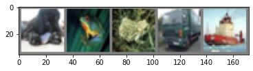
# test CNN-6 using the test data
dataiter = iter(testloader)
images, labels = dataiter.next()

# print images
imshow(torchvision.utils.make_grid(images))
print('GroundTruth: ', ' '.join('%5s' % classes[labels[j]] for j in range(5)))

outputs = net0(images)

_, predicted = torch.max(outputs, 1)

print('Predicted: ', ' '.join('%5s' % classes[predicted[j]]
                              for j in range(5)))

correct = 0
total = 0
# since we're not training, we don't need to calculate the gradients for our outputs
with torch.no_grad():
    for data in testloader:
        images, labels = data
        # calculate outputs by running images through the network
        outputs = net0(images)
        # the class with the highest energy is what we choose as prediction
        _, predicted = torch.max(outputs.data, 1)
        total += labels.size(0)
        correct += (predicted == labels).sum().item()

print('Accuracy of the network on the 10000 test images: %d %%' % (
    100 * correct / total))

GroundTruth:    cat  ship  ship plane  frog
Predicted:   frog   car plane plane  deer
Accuracy of the network on the 10000 test images: 56 %
# Train CNN-7 classifier
class Net(nn.Module):
    def __init__(self):
        super().__init__()
        self.conv1 = nn.Conv2d(3, 6, 5)
        self.pool = nn.MaxPool2d(2, 2)
        self.conv2 = nn.Conv2d(6, 16, 5)
        self.fc1 = nn.Linear(16 * 5 * 5, 120)
        self.fc2 = nn.Linear(120, 84)
        self.fc3 = nn.Linear(84, 10)

    def forward(self, x):
        x = self.pool(F.relu(self.conv1(x)))
        x = self.pool(F.relu(self.conv2(x)))
        x = torch.flatten(x, 1) # flatten all dimensions except batch
        x = F.relu(self.fc1(x))
        x = F.relu(self.fc2(x))
        x = self.fc3(x)
        return x


net1 = Net()
criterion = nn.CrossEntropyLoss()
optimizer = optim.SGD(net1.parameters(), lr=0.001, momentum=0.9)
for epoch in range(2):  # loop over the dataset multiple times

    running_loss = 0.0
    for i, data in enumerate(trainloader, 0):
        # get the inputs; data is a list of [inputs, labels]
        inputs, labels = data

        # zero the parameter gradients
        optimizer.zero_grad()

        # forward + backward + optimize
        outputs = net1(inputs)
        loss = criterion(outputs, labels)
        loss.backward()
        optimizer.step()

        # print statistics
        running_loss += loss.item()
        if i % 2000 == 1999:    # print every 2000 mini-batches
            print('[%d, %5d] loss: %.3f' %
                  (epoch + 1, i + 1, running_loss / 2000))
            running_loss = 0.0

print('Finished Training')
[1,  2000] loss: 2.169
[1,  4000] loss: 1.817
[1,  6000] loss: 1.665
[1,  8000] loss: 1.578
[1, 10000] loss: 1.504
[2,  2000] loss: 1.440
[2,  4000] loss: 1.403
[2,  6000] loss: 1.366
[2,  8000] loss: 1.333
[2, 10000] loss: 1.292
Finished Training
Test the cnn model
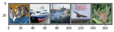
#Test CNN-7 using test data
dataiter = iter(testloader)
images, labels = dataiter.next()

# print images
imshow(torchvision.utils.make_grid(images))
print('GroundTruth: ', ' '.join('%5s' % classes[labels[j]] for j in range(4)))

outputs = net1(images)

_, predicted = torch.max(outputs, 1)

print('Predicted: ', ' '.join('%5s' % classes[predicted[j]]
                              for j in range(4)))

correct = 0
total = 0
# since we're not training, we don't need to calculate the gradients for our outputs
with torch.no_grad():
    for data in testloader:
        images, labels = data
        # calculate outputs by running images through the network
        outputs = net1(images)
        # the class with the highest energy is what we choose as prediction
        _, predicted = torch.max(outputs.data, 1)
        total += labels.size(0)
        correct += (predicted == labels).sum().item()

print('Accuracy of the network on the 10000 test images: %d %%' % (
    100 * correct / total))

GroundTruth:    cat  ship  ship plane
Predicted:    cat  ship  ship  ship
Accuracy of the network on the 10000 test images: 51 %
#Train CNN-8 classifier
class Net(nn.Module):
    def __init__(self):
        super().__init__()
        self.conv1 = nn.Conv2d(3, 200, 5)
        self.pool = nn.MaxPool2d(2, 2)
        self.conv2 = nn.Conv2d(200, 300, 5)
        self.conv3 = nn.Conv2d(300, 400, 5)
        self.fc1 = nn.Linear(400* 1 * 1, 200)
        self.fc2 = nn.Linear(200, 400)
        self.fc3 = nn.Linear(400, 10)

    def forward(self, x):
        x = self.pool(F.relu(self.conv1(x)))
        x = self.pool(F.relu(self.conv2(x)))
        x = F.relu(self.conv3(x))
        x = torch.flatten(x, 1) # flatten all dimensions except batch
        x = F.relu(self.fc1(x))
        x = F.relu(self.fc2(x))
        x = self.fc3(x)
        return x


net2 = Net()
criterion = nn.CrossEntropyLoss()
optimizer = optim.SGD(net2.parameters(), lr=0.001, momentum=0.9)
for epoch in range(2):  # loop over the dataset multiple times

    running_loss = 0.0
    for i, data in enumerate(trainloader, 0):
        # get the inputs; data is a list of [inputs, labels]
        inputs, labels = data

        # zero the parameter gradients
        optimizer.zero_grad()

        # forward + backward + optimize
        outputs = net2(inputs)
        loss = criterion(outputs, labels)
        loss.backward()
        optimizer.step()

        # print statistics
        running_loss += loss.item()
        if i % 2000 == 1999:    # print every 2000 mini-batches
            print('[%d, %5d] loss: %.3f' %
                  (epoch + 1, i + 1, running_loss / 2000))
            running_loss = 0.0

print('Finished Training')
[1,  2000] loss: 2.081
[1,  4000] loss: 1.659
[1,  6000] loss: 1.486
[1,  8000] loss: 1.362
[1, 10000] loss: 1.254
[2,  2000] loss: 1.154
[2,  4000] loss: 1.100
[2,  6000] loss: 1.043
[2,  8000] loss: 1.001
[2, 10000] loss: 0.967
Finished Training
#Test CNN-8 classifier on test data
dataiter = iter(testloader)
images, labels = dataiter.next()

# print images
imshow(torchvision.utils.make_grid(images))
print('GroundTruth: ', ' '.join('%5s' % classes[labels[j]] for j in range(5)))

outputs = net2(images)

_, predicted = torch.max(outputs, 1)

print('Predicted: ', ' '.join('%5s' % classes[predicted[j]]
                              for j in range(5)))

correct = 0
total = 0
# since we're not training, we don't need to calculate the gradients for our outputs
with torch.no_grad():
    for data in testloader:
        images, labels = data
        # calculate outputs by running images through the network
        outputs = net2(images)
        # the class with the highest energy is what we choose as prediction
        _, predicted = torch.max(outputs.data, 1)
        total += labels.size(0)
        correct += (predicted == labels).sum().item()

print('Accuracy of the network on the 10000 test images: %d %%' % (
    100 * correct / total))
GroundTruth:    cat  ship  ship plane  frog
Predicted:    cat  ship  ship plane  frog
Accuracy of the network on the 10000 test images: 66 %
3.1 Test results
The table below presents the model accuracies and losses of each classifer in this section. It turns out that, CNN-8,the 3 convolutional layers with 3 fully connected layers performed better the other two models with an accuracy rate of 66% and a loss of 0.967. Therefore, CNN-8 is the optimal classifier using pytorch.
model2 = {'Model': ['CNN-6', 'CNN-7', 'CNN-8'],
       'Accuracy': [0.56, 0.51, 0.66],
       'Loss': [1.238, 1.292, 0.967]}
modeldata1 = DataFrame(model2)   # creating DataFrame from dictionary
modeldata1
| Model | Accuracy | Loss | |
|---|---|---|---|
| 0 | CNN-6 | 0.56 | 1.238 |
| 1 | CNN-7 | 0.51 | 1.292 |
| 2 | CNN-8 | 0.66 | 0.967 |
A classification report of each class based on the optimal model, CNN-8, is presented below.
# prepare to count predictions for each class
correct_pred = {classname: 0 for classname in classes}
total_pred = {classname: 0 for classname in classes}

# again no gradients needed
with torch.no_grad():
    for data in testloader:
        images, labels = data
        outputs = net2(images)
        _, predictions = torch.max(outputs, 1)
        # collect the correct predictions for each class
        for label, prediction in zip(labels, predictions):
            if label == prediction:
                correct_pred[classes[label]] += 1
            total_pred[classes[label]] += 1


# print accuracy for each class
for classname, correct_count in correct_pred.items():
    accuracy = 100 * float(correct_count) / total_pred[classname]
    print("Accuracy for class {:5s} is: {:.1f} %".format(classname,
                                                   accuracy))
Accuracy for class plane is: 78.8 %
Accuracy for class car   is: 78.9 %
Accuracy for class bird  is: 42.1 %
Accuracy for class cat   is: 49.6 %
Accuracy for class deer  is: 57.8 %
Accuracy for class dog   is: 66.0 %
Accuracy for class frog  is: 62.9 %
Accuracy for class horse is: 65.2 %
Accuracy for class ship  is: 82.1 %
Accuracy for class truck is: 77.8 %
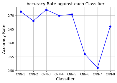
Visualization of accuracies against models
model3 = {'Model': ['CNN-1', 'CNN-2', 'CNN-3', 'CNN-4', 'CNN-5','CNN-6','CNN-7','CNN-8'],
       'Accuracy': [0.7133, 0.6800, 0.7199, 0.6993,0.7030,0.5600, 0.5100, 0.6600],
       'Loss': [0.8540, 0.9267, 0.8247, 0.8775,0.8773,1.2380, 1.2920, 0.9670]}
modeldata3 = DataFrame(model3)   # creating DataFrame from dictionary
modeldata3
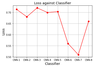
| Model | Accuracy | Loss | |
|---|---|---|---|
| 0 | CNN-1 | 0.7133 | 0.8540 |
| 1 | CNN-2 | 0.6800 | 0.9267 |
| 2 | CNN-3 | 0.7199 | 0.8247 |
| 3 | CNN-4 | 0.6993 | 0.8775 |
| 4 | CNN-5 | 0.7030 | 0.8773 |
| 5 | CNN-6 | 0.5600 | 1.2380 |
| 6 | CNN-7 | 0.5100 | 1.2920 |
| 7 | CNN-8 | 0.6600 | 0.9670 |
%matplotlib inline

Classifier = ['CNN-1','CNN-2','CNN-3','CNN-4','CNN-5','CNN-6','CNN-7','CNN-8']
Accuracy_Rate = [0.7133,0.6800,0.7199,0.6993,0.7030,0.5600,0.5100,0.6600]

plt.plot(Classifier, Accuracy_Rate, color='blue', marker='o')
plt.title('Accuracy Rate against Classifier', fontsize=14)
plt.xlabel('Classifier', fontsize=14)
plt.ylabel('Accuracy Rate', fontsize=14)
plt.grid(True)
plt.show()
Classifier = ['CNN-1','CNN-2','CNN-3','CNN-4','CNN-5','CNN-6','CNN-7','CNN-8']
Loss = [0.8540,0.9267,0.8247,0.8775,0.8773,1.2380,1.2920,0.9670]

plt.plot(Classifier, Accuracy_Rate, color='red', marker='o')
plt.title('Loss against Classifier', fontsize=14)
plt.xlabel('Classifier', fontsize=14)
plt.ylabel('Loss', fontsize=14)
plt.grid(True)
plt.show()
Contributions, challenges and conclusions
In this project, I used a referece code (references stated above) and lecture notes to build an image classifier for the CIFAR-10 dataset. 8 different classifiers were built using different tuning parameter values and network size. The purpose of this is to be able to select an optimal predictive model for the CIFAR-10 dataset. Detail reports of my results are provided to enhance understanding.
The first challenge I encounter in this project is how to determine the optimal parameter value, and the second challenge has to do with pytorch. Training a classifier with pytorch with many layers is computationally inefficient since it takes long time to generate the results.
In conclusion, from my results, it’s clear that the optimal model for the data under tensorflow is CNN-3 and that of pytorch is CNN-8.
Wisdom Aselisewine
Ph.D Student of Statistics
My research interests include Machine Learning Methods, Survival Analysis, Statistical Computing, and Actuarial Science.